Functions
Functions are additional operations that can be employed when calculating values for YSLD parameters. In most cases, a value for a parameter can be the output (result) of a function.
Functions can be used in most places in a style document.
Syntax
Functions aren’t a parameter to itself, but instead are used as a part of the values of a parameter, or indeed in any expression. So the syntax is very general, for example:
<parameter>: ${<function>}
Functions are evaluated at rendering time, so the output is passed as the parameter value and then rendered accordingly.
List of functions
A reference list of functions can be found in the GeoServer User Manual and is also available in raw form in the GeoTools User Manual Function List.
The functions can be broken up loosely into categories such as geometric, math, and string functions.
Theming functions
There are three important functions that are often easier to use for theming than using rules, and can vastly simplify your style documents: Recode, Categorize, and Interpolate.
Recode: Attribute values are directly mapped to styling properties:
recode(attribute,value1,result1,value2,result2,value3,result3,...)
This is equivalent to creating multiple rules with similar filters:
rules:
- ...
  filter: ${attribute = value1}
  - ...
    <property>: result1
- ...
  filter: ${attribute = value2}
  - ...
    <property>: result2
- ...
  filter: ${attribute = value3}
  - ...
    <property>: result3
Categorize: Categories are defined using minimum and maximum ranges, and attribute values are sorted into the appropriate category:
categorize(attribute,category0,value1,category1,value2,category2,...,belongsTo)
This would create a situation where the attribute value, if less than value1 will be given the result of category0; if between value1 and value2, will be given the result of category1; if between value2 and value3, will be given the result of category2, etc. Values must be in ascending order.
The belongsTo argument is optional, and can be either succeeding or preceding. It defines which interval to use when the lookup value equals the attribute value. If the attribute value is equal to value1 and suceeding is used, then the result will be category1. If preceding is used then the result will be category0. The default is succeeding.
This is equivalent to creating the following multiple rules:
rules:
- ...
  filter: ${attribute < value1}
  - ...
    <property>: category0
- ...
  filter: ${attribute >= value1 AND attribute < value2}
  - ...
    <property>: category1
- ...
  filter: ${attribute >= value2}
  - ...
    <property>: category2
Interpolate: Used to smoothly theme quantitative data by calculating a styling property based on an attribute value. This is similar to Categorize, except that the values are continuous and not discrete:
interpolate(attribute,value1,entry1,value2,entry2,...,mode,method)
This would create a situation where the attribute value, if equal to value1 will be given the result of entry1; if halfway between value1 and value2 will be given a result of halfway in between entry1 and entry2; if three-quarters between value1 and value2 will be given a result of three-quarters in between entry1 and entry2, etc.
The mode argument is optional, and can be either linear, cosine, or cubic. It defines the interpolation algorithm to use, and defaults to linear.
The method argument is optional, and can be either numeric or color. It determines whether entry1, entry2, … are numbers or colors, and defaults to numeric.
There is no equivalent to this function in vector styling. The closest to this in raster styling is the color ramp.
The three theming functions can be neatly summarized by this table:
Function |
Type of input |
Type of output |
|---|---|---|
Recode |
Discrete |
Discrete |
Categorize |
Continuous |
Discrete |
Interpolate |
Continuous |
Continuous |
Examples
Display rotated arrows at line endpoints
The startPoint(geom) and endPoint(geom) functions take a geometry as an argument and returns the start and end points of the geometry respectively. The startAngle(geom) and endAngle(geom) functions take a geometry as an argument and return the angle of the line terminating at the start and end points of the geometry respectively. These functions can be used to display an arrow at the end of a line geometry, and rotate it to match the direction of the line:
feature-styles:
- rules:
  - symbolizers:
      - line:
          stroke-width: 1
      - point:
          geometry: ${endPoint(geom)}
          rotation: ${endAngle(geom)}
          size: 24
          symbols:
          - mark:
              shape: 'shape://carrow'
              fill-color: '#000000'
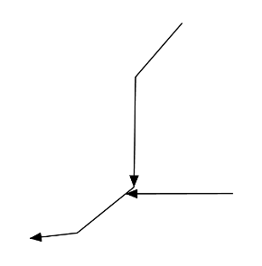
Endpoint arrows
Drop shadow
The offset(geom, x, y) function takes a geometry and two values, and displaces the geometry by those values in the x and y directions. This can be used to create a drop-shadow effect:
feature-styles:
- name: shadow
  rules:
  - symbolizers:
    - polygon:
        stroke-width: 0.0
        fill-color: '#000000'
        fill-opacity: 0.75
        geometry: ${offset(geom, 0.0001, -0.0001)}
- name: fill
  rules:
  - symbolizers:
    - polygon:
      stroke-width: 0.0
      fill-color: '#00FFFF'
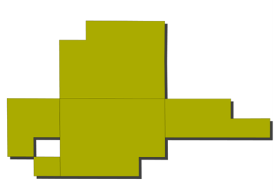
Drop shadow
Different-colored outline
The buffer(geom, buffer) function takes a geometry and a value as arguments, and returns a polygon geometry with a boundary equal to the original geometry plus the value. This can be used to generate an extended outline filled with a different color, for example to style a shoreline:
feature-styles:
- name: shoreline
  rules:
  - polygon:
      fill-color: '#00BBFF'
      geometry: ${buffer(geom, 0.00025)}
- name: land
  rules:
  - polygon:
      fill-color: '#00DD00'
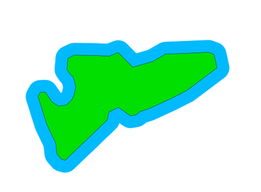
Buffered outline
See also:
Display vertices of a line
The vertices(geom) function takes a geometry and returns a collection of points representing the vertices of the geometry. This can be used to convert a polygon or line geometry into a point geometry:
point:
  geometry: vertices(geom)
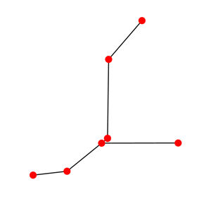
Endpoint arrows
See also:
Angle between two points
The atan2(x, y) function calculates the arctangent of (y/x) and so is able to determine the angle (in radians) between two points. This function uses the signs of the x and y values to determine the computed angle, so it is preferable over atan(). The getX(point_geom) and getY(point_geom) extracts the x and y ordinates from a geometry respectively, while toDegrees(value) converts from radians to degrees:
point:
  symbols:
  - mark:
      shape: triangle
  rotation: ${toDegrees(atan2(
    getX(startPoint(the_geom))-getX(endPoint(the_geom)),
    getY(startPoint(the_geom))-getY(endPoint(the_geom))))}
See also:
Scale objects based on a large range of values
The log(value) function returns the natural logarithm of the provided value. Use log(value)/log(base) to specify a different base.
For example, specifying log(population)/log(2) will make the output increase by 1 when the value of population doubles. This allows one to display relative sizes on a consistent scale while still being able to represent very small and very large populations:
point:
  symbols:
  - mark:
      shape: circle
  size: ${log(population)/log(2)}
See also:
Combine several strings into one
The Concatenate(string1, string2, ...) function takes any number of strings and combines them to form a single string. This can be used to display more than one attribute within a single label:
text:
  label: ${Concatenate(name, ', ', population)}
Capitalize words
The strCapitalize(string) function takes a single string and capitalizes the first letter of each word in the string. This could be used to capitalize labels created from lower case text:
text:
  label: ${strCapitalize(name)}
See also:
Color based on discrete values
In certain cases, theming functions can be used in place of filters to produce similar output much more simply. For example, the Recode function can take an attribute and output a different value based on an attribute value. So instead of various filters, the entire constructions can be done in a single line. For example, this could be used to color different types of buildings:
feature-styles:
- name: name
  rules:
  - symbolizers:
    - polygon:
        fill-color:
          ${recode(zone,
          'I-L', '#FF7700',
          'I-H', '#BB6600',
          'C-H', '#0077BB',
          'C-R', '#00BBDD',
          'C-C', '#00DDFF',
          '', '#777777')}
In the above example, the attribute is zone , and then each subsequent pair consists of an attribute value followed by a color.
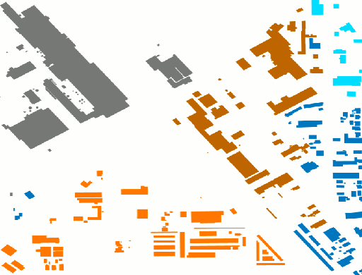
Recode Function
Color based on categories
The Categorize function returns a different value depending on which range (category) an attribute value matches. This can also make a style much more simple by reducing the number of filters. This example uses categorize to color based on certain values of the YEARBLT attribute:
feature-styles:
- name: name
  rules:
  - symbolizers:
     - polygon:
        stroke-color: '#000000'
        stroke-width: 0.5
        fill-color:
          ${categorize(YEARBLT, '#DD4400',
          1950,'#AA4400',
          1960,'#886600',
          1970,'#668800',
          1980,'#44BB00',
          1990,'#22DD00',
          2000,'#00FF00')}
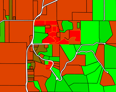
Categorize Function
Choropleth map
The interpolate function can be used to create a continuous set of values by interpolating between attribute values. This can be used to create a choropleth map which shows different colors for regions based on some continuous attribute such as area or population:
feature-styles:
- name: name
  rules:
  - title: fill-graphic
    symbolizers:
    - polygon:
        stroke-width: 1
        fill-color: ${interpolate(PERSONS, 0.0, '#00FF00', 1e7,'#FF0000', 'color')}
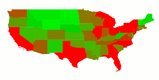
Choropleth Map